Reading Data and Fitting with Pandas

Questions

How do I use pandas to load and inspect experimental data from a CSV file?
How do I plot and fit data held in a DataFrame?

Objectives

Load a CSV file with pandas.read_csv and inspect it with .head() and .describe().
Access columns by name and pass them to matplotlib and curve_fit.
Report fit parameters and uncertainties from the covariance matrix.

Why pandas?

Pandas is a library that behaves a lot like NumPy with arrays of numbers, but instead of using column (or row) indices to reference the data you can use column names (you can do this with NumPy too, but it’s more convoluted). Pandas reads a CSV file into a DataFrame - a table where each column has a name and a type. You can then refer to columns by name making your code easier to read.

Example problem: Galileo’s ramp experiment

Galileo rolled a ball off a table edge and measured the horizontal distance D it traveled as a function of the release height H on the ramp. Theory predicts:

\[D = k \sqrt{H}\]

where k depends on the table height and gravitational acceleration. Load the data, plot it, and find k with its uncertainty.

Worked solution

import pandas as pd
import numpy as np
import matplotlib.pyplot as plt
from scipy.optimize import curve_fit

df = pd.read_csv("data/galileo_ramp.csv", comment="#")
print(df.head())
print(df.describe())

     D     H
0  573  1000
1  534   800
2  495   600
3  451   450
4  395   300
                D            H
count    7.000000     7.000000
mean   434.000000   492.857143
std    113.300485   327.144937
min    253.000000   100.000000
25%    366.000000   250.000000
50%    451.000000   450.000000
75%    514.500000   700.000000
max    573.000000  1000.000000

The DataFrame columns are named from the header row. Select them by name to pass to plotting and fitting functions:

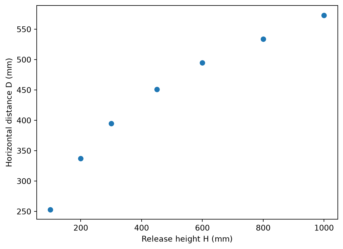
plt.errorbar(df["H"], df["D"], fmt="o")
plt.xlabel("Release height H (mm)")
plt.ylabel("Horizontal distance D (mm)")
plt.show()

Figure 1: Horizontal distance D versus release height H from Galileo’s ramp experiment

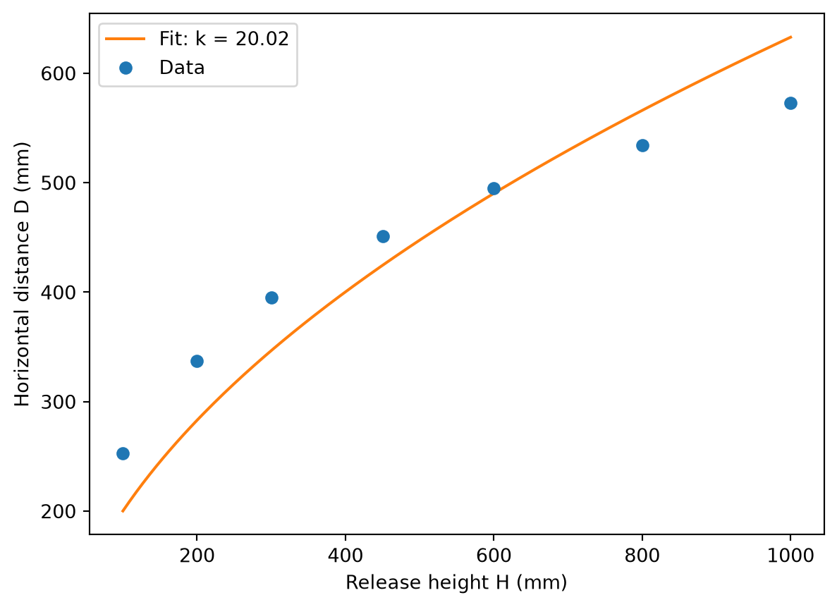
Define the model and fit. curve_fit accepts any array-like, including a pandas Series, as data:

def model(H, k):
    return k * np.sqrt(H)

popt, pcov = curve_fit(model, df["H"], df["D"])
k_fit = popt[0]
k_err = np.sqrt(pcov[0, 0])

print(f"k = {k_fit:.3f} ± {k_err:.3f} mm^(1/2)")

k = 20.015 ± 0.804 mm^(1/2)

H_range = np.linspace(df["H"].min(), df["H"].max(), 200)

plt.errorbar(df["H"], df["D"], fmt="o", label="Data")
plt.plot(H_range, model(H_range, k_fit), label=f"Fit: k = {k_fit:.2f}")
plt.xlabel("Release height H (mm)")
plt.ylabel("Horizontal distance D (mm)")
plt.legend()
plt.show()

Figure 2: Horizontal distance D versus sqrt(H) with the best-fit model overlaid

Selecting subsets with pandas

A common task is filtering rows before fitting — for example, keeping only measurements above a threshold height:

df_high = df[df["H"] >= 600]
print(f"{len(df_high)} rows with H ≥ 600 mm")

popt_high, pcov_high = curve_fit(model, df_high["H"], df_high["D"])
print(f"k (H ≥ 600) = {popt_high[0]:.3f} ± {np.sqrt(pcov_high[0,0]):.3f}")

3 rows with H ≥ 600 mm
k (H ≥ 600) = 18.895 ± 0.584

Boolean indexing (df[condition]) returns a new DataFrame with only the matching rows — the index, column names, and types are all preserved.

Key Points

pd.read_csv("file.csv", comment="#") skips header comment lines and names columns from the first non-comment row.
Access columns by name: df["H"] is a Series that works anywhere NumPy arrays are accepted.
.head(), .describe(), and .dtypes are quick ways to inspect a DataFrame before plotting or fitting.
Use boolean indexing df[df["col"] > value] to filter rows before analysis.