import numpy as np
import matplotlib.pyplot as plt
from scipy.optimize import curve_fit

def reduced_chi2(residuals, sigma, n_params):
return np.sum((residuals / sigma)**2) / (len(residuals) - n_params)Fitting with an Offset
NoteQuestions
- Should I add an offset parameter to my fit when the theory says there isn’t one?
- What does the fitted offset tell me about my experiment?
- What does an extra offset parameter cost?
NoteObjectives
- Explain why a fit with an offset is often more reliable than a fit forced through zero.
- Recognise two common causes of an offset: a zero error in a measurement, and a model that only applies over part of the range.
- Use the fitted offset and its uncertainty to test the model.
- Describe what an offset cannot correct, and when to leave it out.
Why add an offset?
Many physics models pass through the origin. Ohm’s law \(V = IR\), Hooke’s law \(x = F/k\), and the pendulum relation \(T^2 = 4\pi^2 L / g\) all predict zero output for zero input. It is tempting to fit them exactly as written, with a single slope parameter. In practice, fitting with an extra offset parameter is often the better choice, for the following reasons.
- Measurements often have a zero error. A meter that reads 0.02 V with its leads shorted, a balance that was not tared, or a length measured to the wrong point on an object all add a constant to every reading. This is a measurement error, not physics, but a fit forced through zero cannot account for it, and the slope absorbs the error instead.
- The model may only apply over part of the range. Real systems often depart from the simple model at small x: a spring with initial tension does not stretch until the load passes a threshold, and a lamp filament is cooler at low current. A fit forced through zero requires the model to hold all the way to \(x = 0\), so the region where the model fails determines the slope. With an offset, the slope is determined by the data in the range where the model holds.
- The offset is a test of the model. If the fitted offset is consistent with zero within its uncertainty, the data support the model as written. If it is not, something is missing: a zero error, a failure of the model, or a systematic effect you had not considered. A fit forced through zero cannot tell you any of this.
- The two possible mistakes have different consequences. Including an offset that is not needed makes the slope uncertainty larger, which is cautious but still correct. Leaving out an offset that is needed shifts the slope and gives an uncertainty that is too small, so the result is wrong and appears precise.
The examples below show each of these.
Example 1: a zero error in the measurement
A pendulum’s length should be measured from the pivot to the centre of the bob. In this data set the lengths were measured to the top of the bob, which has a radius of 1.25 cm, so every length is 1.25 cm too short. The periods were timed with \(\sigma_T = 0.005\) s and the length uncertainty is negligible.
Squaring the period gives a model that is linear in \(L\):
\[ T^2 = \frac{4\pi^2}{g} L \]
The uncertainty in \(T^2\) is \(\sigma_{T^2} = 2T\sigma_T\).
L = np.array([0.2, 0.3, 0.4, 0.5, 0.6, 0.7, 0.8, 0.9, 1.0])   # metres
T = np.array([0.926, 1.116, 1.292, 1.441, 1.560,
              1.687, 1.809, 1.915, 2.018])                    # seconds
T_err = 0.005

T2 = T**2
T2_err = 2 * T * T_err
Fit two models. The first is the theory as written. The second adds an offset \(L_0\) to the length:
\[ T^2 = a\,(L + L_0) \]
This is the same as a straight line \(T^2 = aL + b\) with \(b = aL_0\). Writing the offset as \(L_0\) means it has units of length, which makes it easier to interpret.
def no_offset(L, a):
    return a * L

def with_offset(L, a, L0):
    return a * (L + L0)

popt0, pcov0 = curve_fit(no_offset, L, T2, sigma=T2_err, absolute_sigma=True)
popt1, pcov1 = curve_fit(with_offset, L, T2, p0=[4, 0],
                         sigma=T2_err, absolute_sigma=True)

for name, model, popt, pcov in [("no offset", no_offset, popt0, pcov0),
                                ("with offset", with_offset, popt1, pcov1)]:
    a, a_err = popt[0], np.sqrt(pcov[0, 0])
    g = 4 * np.pi**2 / a
    g_err = g * a_err / a
    chi2r = reduced_chi2(T2 - model(L, *popt), T2_err, len(popt))
    print(f"{name:12s} g = {g:.3f} ± {g_err:.3f} m/s²   χ²_r = {chi2r:.1f}")

L0, L0_err = popt1[1], np.sqrt(pcov1[1, 1])
print(f"Fitted offset L0 = {L0*1000:.1f} ± {L0_err*1000:.1f} mm")
no offset g = 9.630 ± 0.020 m/s² χ²_r = 4.4
with offset g = 9.837 ± 0.046 m/s² χ²_r = 1.1
Fitted offset L0 = 13.0 ± 2.5 mmplt.errorbar(L, T2 - no_offset(L, *popt0), yerr=T2_err,
marker='o', ls='none', label="no offset")
plt.errorbar(L + 0.01, T2 - with_offset(L, *popt1), yerr=T2_err,
marker='s', ls='none', label="with offset")
plt.axhline(0, color='k', linewidth=0.8)
plt.xlabel("Measured length (m)")
plt.ylabel("$T^2$ − model (s²)")
plt.legend()
plt.show()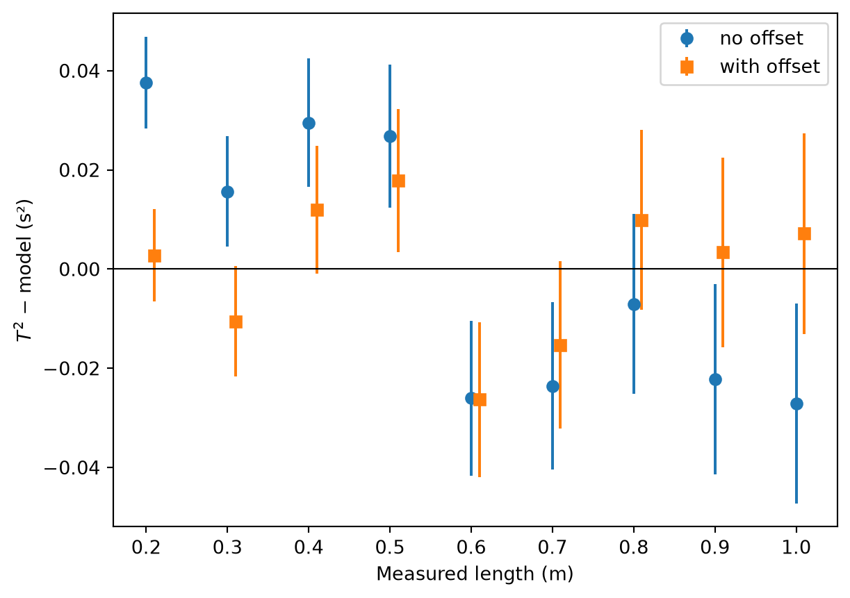
Without the offset, \(g\) is about nine standard deviations below 9.81 m/s², and \(\chi_r^2 \approx 4\). The residuals have a clear slope: positive at short lengths and negative at long lengths. The fit has tilted the line to pass through the origin.
With the offset, \(g\) agrees with 9.81 m/s², \(\chi_r^2 \approx 1\), and the residuals scatter around zero. The fitted offset, about 13 mm, matches the bob radius. The offset was caused by the length measurement, not by the physics, and the fit measured it.
Note that the uncertainty in \(g\) more than doubled. That is the cost of the extra parameter, and it is discussed in Example 3.
Example 2: a model that only applies over part of the range
An extension spring is loaded with masses from 0 to 500 g, and its extension is measured with \(\sigma_x = 1\) mm. Hooke’s law predicts
\[ x = \frac{F}{k}, \qquad F = mg \]
mass = np.array([0.0, 0.05, 0.1, 0.15, 0.2, 0.25,
                 0.3, 0.35, 0.4, 0.45, 0.5])          # kg
x = np.array([0.0009, 0.0001, 0.0189, 0.0429, 0.0693, 0.0925,
              0.1167, 0.1413, 0.1667, 0.1911, 0.2157])  # metres
x_err = np.full_like(x, 0.001)
F = mass * 9.81                                       # newtons

def hooke(F, k):
    return F / k

popt_all, pcov_all = curve_fit(hooke, F, x, p0=[20],
                               sigma=x_err, absolute_sigma=True)
print(f"k = {popt_all[0]:.2f} ± {np.sqrt(pcov_all[0, 0]):.2f} N/m")
print(f"χ²_r = {reduced_chi2(x - hooke(F, *popt_all), x_err, 1):.0f}")
k = 24.19 ± 0.06 N/m
χ²_r = 170\(\chi_r^2\) is far larger than 1. Plotting the data shows why:
F_model = np.linspace(0, 5, 100)
plt.errorbar(F, x, yerr=x_err, marker='o', ls='none', label="Data")
plt.plot(F_model, hooke(F_model, *popt_all), label="Hooke's law, no offset")
plt.xlabel("Force (N)")
plt.ylabel("Extension (m)")
plt.legend()
plt.show()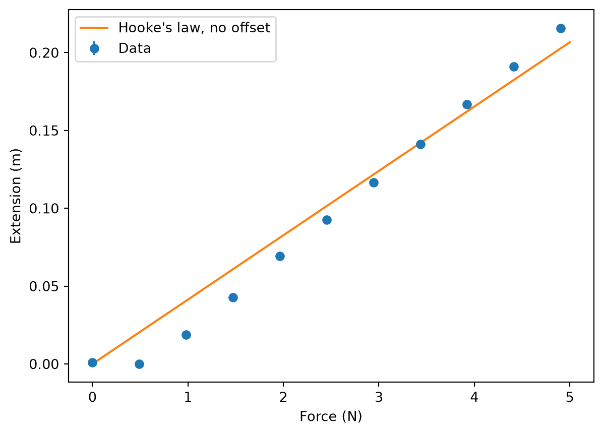
The spring does not stretch at all for the first two loads. Many extension springs are wound with initial tension: the coils press against each other, and the spring only starts to stretch once the load exceeds this tension. Above that point it follows Hooke’s law, but the straight line does not pass through the origin. Hooke’s law in the form \(x = F/k\) does not describe this spring at small loads.
Fit only the points where the spring is stretching (mass ≥ 100 g), with an offset. Writing the offset as a force \(F_0\) gives
\[ x = \frac{F - F_0}{k} \]
where \(F_0\) is the initial tension.
def hooke_offset(F, k, F0):
    return (F - F0) / k

stretching = mass >= 0.1

popt_lin, pcov_lin = curve_fit(hooke_offset, F[stretching], x[stretching],
                               p0=[20, 0.5], sigma=x_err[stretching],
                               absolute_sigma=True)
k, F0 = popt_lin
k_err, F0_err = np.sqrt(np.diag(pcov_lin))
chi2r = reduced_chi2(x[stretching] - hooke_offset(F[stretching], *popt_lin),
                     x_err[stretching], 2)

print(f"k  = {k:.2f} ± {k_err:.2f} N/m")
print(f"F0 = {F0:.3f} ± {F0_err:.3f} N")
print(f"χ²_r = {chi2r:.1f}")
k = 19.95 ± 0.10 N/m
F0 = 0.605 ± 0.014 N
χ²_r = 0.4F_fit = np.linspace(F0, 5, 100)
F_extrap = np.linspace(0, F0, 20)
plt.errorbar(F, x, yerr=x_err, marker='o', ls='none', label="Data")
plt.plot(F_fit, hooke_offset(F_fit, *popt_lin), label="Fit with offset (mass ≥ 100 g)")
plt.plot(F_extrap, hooke_offset(F_extrap, *popt_lin), 'C1--')
plt.axhline(0, color='k', linewidth=0.8)
plt.xlabel("Force (N)")
plt.ylabel("Extension (m)")
plt.legend()
plt.show()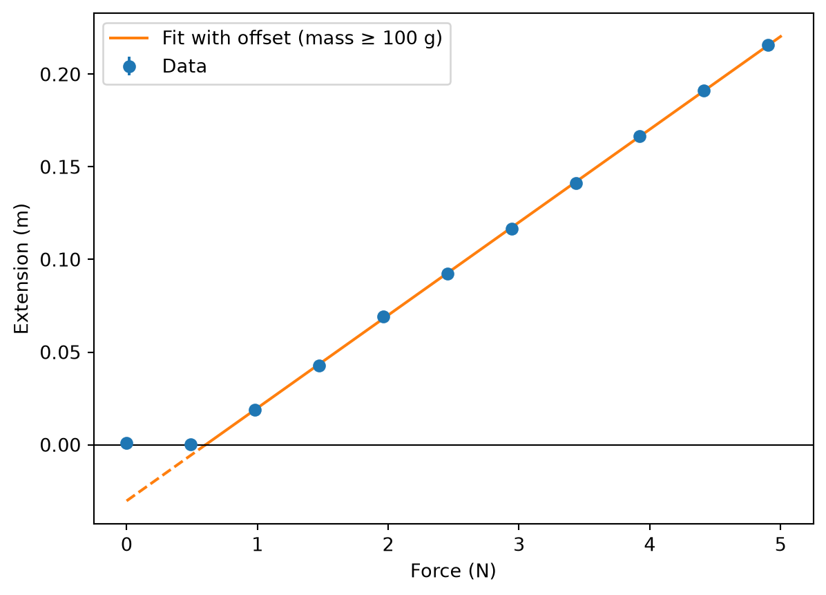
The spring constant is now about 20 N/m instead of 24 N/m, and \(\chi_r^2\) has dropped from about 170 to below 1. The offset has a physical meaning, the initial tension, even though it is not part of Hooke’s law as usually written.
Two separate steps were needed here. The data were restricted to the range where the model applies, and an offset was added so the fit did not have to pass through a point the spring never reaches. Neither step alone is enough: check this in the challenge below.
Example 3: when the offset really is zero
Here is the pendulum experiment repeated with the lengths measured correctly to the centre of the bob:
T_good = np.array([0.893, 1.103, 1.273, 1.419, 1.560,
                   1.681, 1.790, 1.905, 2.001])
T2_good = T_good**2
T2_good_err = 2 * T_good * T_err

popt0g, pcov0g = curve_fit(no_offset, L, T2_good,
                           sigma=T2_good_err, absolute_sigma=True)
popt1g, pcov1g = curve_fit(with_offset, L, T2_good, p0=[4, 0],
                           sigma=T2_good_err, absolute_sigma=True)

for name, popt, pcov in [("no offset", popt0g, pcov0g),
                         ("with offset", popt1g, pcov1g)]:
    a, a_err = popt[0], np.sqrt(pcov[0, 0])
    g = 4 * np.pi**2 / a
    print(f"{name:12s} g = {g:.3f} ± {g * a_err / a:.3f} m/s²")

print(f"Fitted offset L0 = {popt1g[1]*1000:.1f} ± {np.sqrt(pcov1g[1, 1])*1000:.1f} mm")
no offset g = 9.804 ± 0.021 m/s²
with offset g = 9.817 ± 0.045 m/s²
Fitted offset L0 = 0.8 ± 2.4 mmThe fitted offset is consistent with zero, and both fits give the same \(g\). This is evidence that the model without an offset is adequate for these data. Once you have checked this, it is reasonable to report the result from the fit without the offset, which has the smaller uncertainty, and to state that the fitted offset was consistent with zero.
The fit with the offset has twice the uncertainty in \(g\). The reason is that the slope and the offset are correlated: a slightly steeper line with a slightly more negative offset fits the data almost as well. The correlation coefficient from pcov shows this:
corr = pcov1g[0, 1] / np.sqrt(pcov1g[0, 0] * pcov1g[1, 1])
print(f"Correlation between slope and offset: {corr:.2f}")
Correlation between slope and offset: -0.88The correlation is strongest when the data are far from \(x = 0\) compared with their spread. Here the lengths run from 0.2 m to 1.0 m, so the fit has to extrapolate a long way to find the intercept. Measurements over a wider range, particularly closer to \(x = 0\) when the model still applies there, reduce the correlation and the uncertainty.
What an offset cannot do
An offset is a single constant. It can only correct an error that shifts every point by the same amount.
- It cannot correct a scale error. A meter that reads 2% high, or a ruler with the wrong spacing, changes the slope, not the intercept. Only a calibration can find this.
- It cannot correct the wrong shape. If the data curve, adding an offset to a straight line can make the fit look acceptable over a narrow range while the model is still wrong. Always check the residuals for structure, as well as checking \(\chi_r^2\).
- It can hide a failure of the model. In Example 2, fitting all the data with an offset gives a value of \(k\), but the residuals near the threshold show the model does not apply there. The offset should not be used to avoid looking at that region. Decide which range the model applies to, state it in your report, and say why.
- It is not automatically physical. In Example 1 the offset was a measurement error. In Example 2 it was a real property of the spring. The fit cannot tell you which; you have to explain it from your knowledge of the experiment.
When you can measure the zero error directly, for example by reading the meter with its leads shorted or measuring the bob radius, subtract it from the data and compare the result with the fitted offset. The two should agree.
The same reasoning applies to non-linear models. An offset can be added in y, as \(f(x) + c\), or in x, as \(f(x - x_0)\), depending on which measurement might have a zero error.
CautionChallenge
Range and offset
For the spring data in Example 2, fit:
- only the stretching region (mass ≥ 100 g), without an offset, and
- all the data with an offset.
Compare \(k\) and \(\chi_r^2\) with the result from Example 2. Plot the residuals for fit 2. What do they show?
NoteSolution
p_a, c_a = curve_fit(hooke, F[stretching], x[stretching], p0=[20],
                     sigma=x_err[stretching], absolute_sigma=True)
chi2_a = reduced_chi2(x[stretching] - hooke(F[stretching], *p_a),
                      x_err[stretching], 1)

p_b, c_b = curve_fit(hooke_offset, F, x, p0=[20, 0.5],
                     sigma=x_err, absolute_sigma=True)
chi2_b = reduced_chi2(x - hooke_offset(F, *p_b), x_err, 2)

print(f"range only:  k = {p_a[0]:.2f} ± {np.sqrt(c_a[0, 0]):.2f} N/m   χ²_r = {chi2_a:.0f}")
print(f"offset only: k = {p_b[0]:.2f} ± {np.sqrt(c_b[0, 0]):.2f} N/m   χ²_r = {chi2_b:.0f}")
range only: k = 24.13 ± 0.06 N/m χ²_r = 162
offset only: k = 21.36 ± 0.09 N/m χ²_r = 66plt.errorbar(F, x - hooke_offset(F, *p_b), yerr=x_err, marker='o', ls='none')
plt.axhline(0, color='k', linewidth=0.8)
plt.xlabel("Force (N)")
plt.ylabel("Extension − model (m)")
plt.show()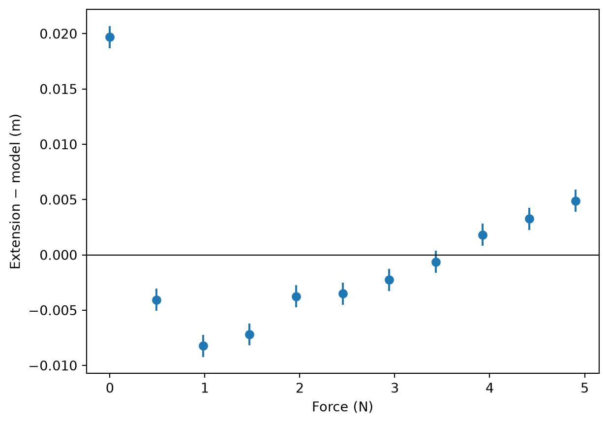
Neither fit is acceptable. Restricting the range without an offset still forces the line through the origin, which this spring never reaches, so \(k\) is still about 24 N/m. Adding an offset but keeping all the points makes the line pass between the flat region and the stretching region. The residuals show a clear pattern: the zero-load point is about 20 mm above the line, the next points are below it, and the residuals then rise steadily with force. \(\chi_r^2\) is still large.
TipKey Points
- Fitting with an offset lets zero errors in the measurements, and regions where the model does not apply, show up in the offset instead of distorting the slope.
- Leaving out a needed offset gives a wrong slope with an uncertainty that is too small. Including an unneeded offset only increases the uncertainty.
- Compare the fitted offset with zero. If it is consistent with zero, the model without an offset is supported; if not, find out why.
- Slope and offset are correlated. The correlation is largest when the data are far from x = 0.
- An offset cannot correct a scale error or the wrong model shape. Always check the residuals and state the range over which you fitted.