Fitting data to models

Questions

How do I find the best-fit parameters for a physical model?
How do I report the uncertainty in those parameters correctly?
How do I know whether a model is a good fit to my data?

Objectives

Use scipy.optimize.curve_fit to fit a model function to experimental data.
Interpret popt and pcov to report parameter values and uncertainties.
Explain the difference between sigma with and without absolute_sigma=True.
Calculate and interpret reduced chi-squared \(\chi_r^2\).
Read a residual plot to diagnose whether a model is appropriate.
Provide initial parameter guesses with p0 when fitting non-linear models.

Data analysis with Python

Many physical systems can be modeled as an equation, which in Python would be represented by a function \(f\). If an appropriate function \(f\) can be found for an experiment we can use the equation to determine physical parameters related to the experiment, and we can use this new model to predict new things about the world. Galileo used this method to calculate the trajectory of cannonballs by rolling them down inclined ramps.

In experimental physics, we constrain these models by designing an experiment with two quantities. The first quantity, that we can control, is the independent variable. The second quantity, that we can measure, is the dependent variable. The relationship between these two quantities can then be used to determine some physical parameters.

A simple example is measuring the path of a moving object. We could guess that the model is moving at a constant speed and design an experiment to find that speed using the model:

\[ s = ut \]

`scipy.optimize.curve_fit` fits a model function to data

scipy provides curve_fit, which takes a model function and a set of measurements and returns the best-fit values of the unknown parameters. Consider measuring the distance travelled by an object moving at constant speed, with time as the controlled variable:

def distance(time, speed):
    """Calculate distance travelled at constant speed."""
    return speed * time

import numpy
from scipy.optimize import curve_fit

derr = 5  # estimated distance measurement error, metres
measured_times = numpy.arange(10, 100, 10)          # seconds
measured_distances = numpy.array([108.2, 220.4, 360.2, 482.8,
        630.6, 793.9, 947.5, 1125.0, 1314.9])       # metres
distance_errors = numpy.ones_like(measured_distances) * derr

popt, pcov = curve_fit(distance, measured_times, measured_distances,
                       sigma=distance_errors, absolute_sigma=True)

print("Speed is {:.4g} m/s".format(popt[0]))
pvar = numpy.diag(pcov)
print("Uncertainty in speed is {:.3g} m/s".format(numpy.sqrt(pvar[0])))

Speed is 13.66 m/s
Uncertainty in speed is 0.0296 m/s

Speed is 13.66 m/s
Uncertainty in speed is 0.0296 m/s

The model function must follow a fixed convention: its first argument must be the array of independent data; any additional arguments are the free parameters that curve_fit will determine; and it must return the predicted dependent values:

def good_model_function(xdata, parameter_1, parameter_2, parameter_3):
    # compute and return the model prediction
    return prediction

`popt` and `pcov`: what `curve_fit` returns

curve_fit always returns exactly two arrays.

popt is a 1D array of the best-fit parameter values, in the same order as the parameters appear in the model function definition. For the single-parameter distance function, popt[0] is the fitted speed.

pcov is the covariance matrix — a square matrix whose size equals the number of parameters. Its diagonal elements are the variances of the fitted parameters:

pvar = numpy.diag(pcov)          # extract the diagonal
uncertainties = numpy.sqrt(pvar) # standard errors

The off-diagonal elements describe how the parameters co-vary: a large off-diagonal value means that if one parameter is nudged upward, another must shift to compensate. For independent parameters the off-diagonals are close to zero.

For a two-parameter fit you can access the covariance matrix elements directly using row and column indices — pcov[0,0] is the variance of the first parameter, pcov[1,1] the variance of the second, and pcov[0,1] their covariance.

`sigma` and `absolute_sigma`: getting uncertainties right

The sigma keyword passes your per-point measurement uncertainties to curve_fit. The absolute_sigma keyword controls how those values are interpreted, and the difference matters enormously for the reported parameter uncertainties.

Without absolute_sigma=True (the default), curve_fit treats sigma as relative weights only. After finding the best-fit parameters it rescales the covariance matrix so that the reduced chi-squared (see below) is exactly 1. The reported uncertainties are then self-consistent — they reflect the scatter of the data around the model — but they are not in the physical units of your measurement errors. If your ruler really is accurate to ±5 m, the default mode ignores that.

With absolute_sigma=True, the sigma values are taken at face value as physically meaningful standard deviations. The covariance matrix is not rescaled, so the reported uncertainties are in the same units as your measurement errors and can be directly compared to your experimental precision.

In experimental physics you almost always want absolute_sigma=True. The difference in practice:

# Without absolute_sigma — sigma used only as weights, uncertainties rescaled
popt_rel, pcov_rel = curve_fit(distance, measured_times, measured_distances,
                               sigma=distance_errors)
print("Uncertainty (relative sigma):  {:.3g} m/s".format(numpy.sqrt(pcov_rel[0,0])))

# With absolute_sigma — uncertainties are in physical units
popt_abs, pcov_abs = curve_fit(distance, measured_times, measured_distances,
                               sigma=distance_errors, absolute_sigma=True)
print("Uncertainty (absolute sigma):  {:.3g} m/s".format(numpy.sqrt(pcov_abs[0,0])))

Uncertainty (relative sigma):  0.31 m/s
Uncertainty (absolute sigma):  0.0296 m/s

Uncertainty (relative sigma):  0.31 m/s
Uncertainty (absolute sigma):  0.0296 m/s

The two fits find the same best-fit speed, but the reported uncertainties differ because the default mode assumed the model was perfect and used the residuals to estimate errors, while absolute_sigma=True used the ruler precision you provided. The correct choice depends on which you trust more — but for physics experiments where you have a calibrated measurement process, always use absolute_sigma=True.

Challenge

Predicting with the model

Use the fitted model to predict the distance travelled after 10 s and after 100 s.

Solution

Always call the model function to make predictions — never rewrite the equation or hard-code the fitted value. If you later improve the fit, all predictions update automatically:

d10  = distance(10,  popt[0])
d100 = distance(100, popt[0])
print("After  10 s: {:.4g} m".format(d10))
print("After 100 s: {:.4g} m".format(d100))

After  10 s: 136.6 m
After 100 s: 1366 m

After  10 s: 136.6 m
After 100 s: 1366 m

`curve_fit` works with multiple parameters

What if the object was actually accelerating? The model becomes

\[ s = ut + \frac{1}{2} a t^2 \]

Add acceleration as a second parameter, re-run the fit, and curve_fit finds both simultaneously:

def distance_with_acceleration(time, speed, acceleration):
    """Distance under constant acceleration from rest."""
    return speed * time + 0.5 * acceleration * time**2

popt2, pcov2 = curve_fit(distance_with_acceleration,
                         measured_times, measured_distances,
                         sigma=distance_errors, absolute_sigma=True)

print("Initial speed:  {:.4g} ± {:.3g} m/s".format(
      popt2[0], numpy.sqrt(pcov2[0, 0])))
print("Acceleration:   {:.4g} ± {:.3g} m/s²".format(
      popt2[1], numpy.sqrt(pcov2[1, 1])))

Initial speed:  10.26 ± 0.119 m/s
Acceleration:   0.09589 ± 0.00325 m/s²

Initial speed:  10.26 ± 0.119 m/s
Acceleration:   0.09589 ± 0.00325 m/s²

The data are synthetic, generated with initial speed 10.86 m/s and acceleration 0.1 m/s². The constant-speed model fitted earlier returned speed ≈ 13.7 m/s — it inflated the speed estimate to compensate for the missing acceleration term.

Always plot your data and model fits

Before trusting any numerical result, plot the data with error bars and overlay the model. A visual check catches problems — wrong model shape, outliers, data entry errors — that numbers alone miss:

import matplotlib.pyplot as plt
plt.style.use("seaborn-v0_8-whitegrid")
plt.figure(figsize=(8, 6))
plt.errorbar(measured_times, measured_distances, yerr=distance_errors,
             marker='o', linestyle='none', label="measured data")
plt.plot(measured_times, distance(measured_times, popt[0]),
         label='$s=ut$')
plt.plot(measured_times,
         distance_with_acceleration(measured_times, popt2[0], popt2[1]),
         label=r'$s=ut+\frac{1}{2}at^2$')
plt.legend(fontsize=14)
plt.xlabel("Time (s)")
plt.ylabel("Distance (m)")
plt.show()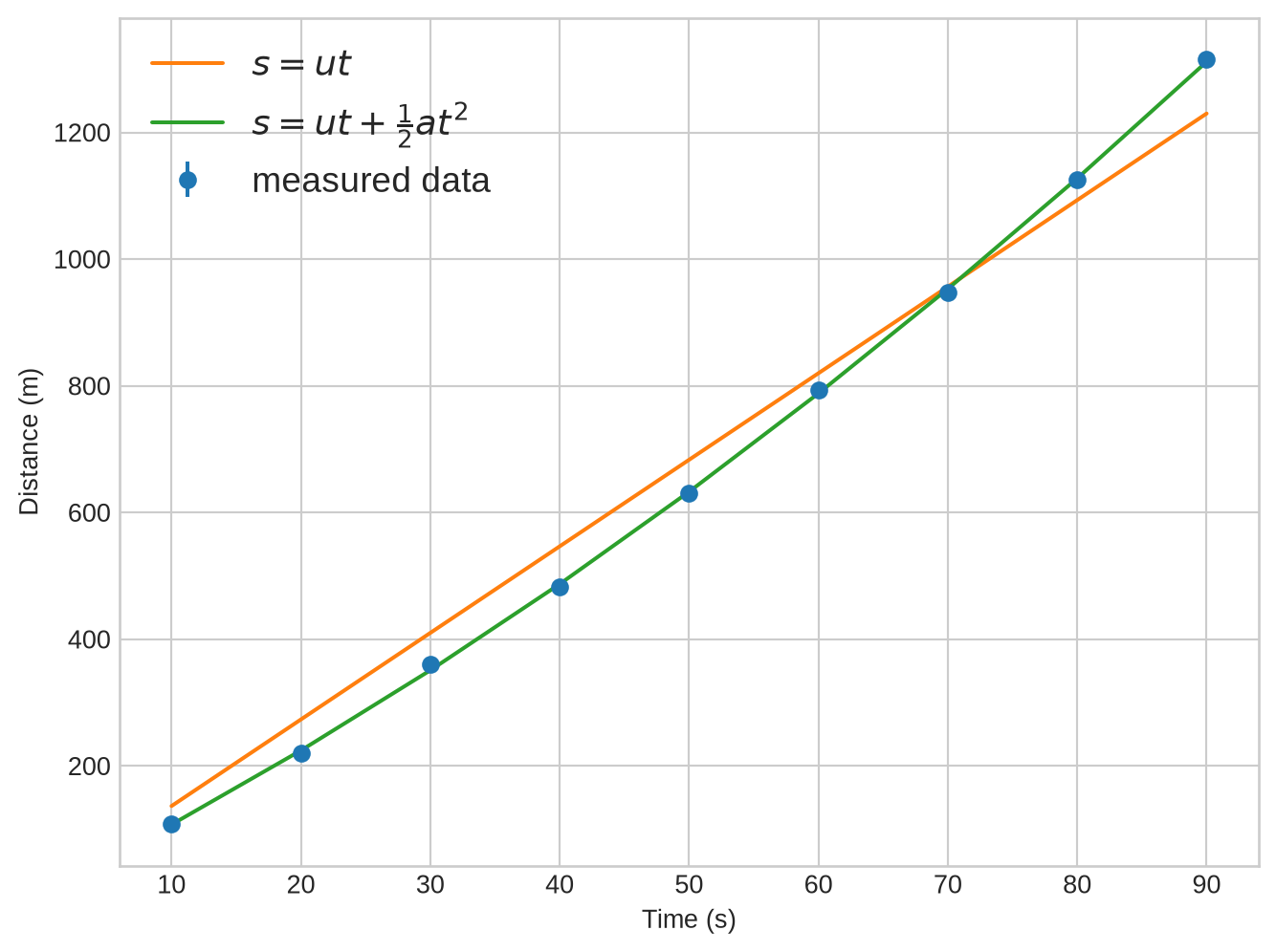

Figure 1: Distance versus time showing the measured data with error bars and two model fits: a constant-velocity model and a constant-acceleration model

Residual plots diagnose model quality

A residual is the difference between a model prediction and the measured value:

\[\text{residual}_i = f(x_i) - y_i\]

Plotting residuals against the independent variable amplifies any systematic deviation that is hard to see on the data plot. A good model produces residuals that:

scatter randomly around zero with no visible trend,
have a spread comparable to the measurement uncertainties.

A trend in the residuals — values that drift positive then negative as the independent variable increases, or form a curve — means the model is missing something. It is not capturing the shape of the data.

plt.figure(figsize=(8, 4))
plt.axhline(0, color='k', lw=0.8, ls='--')
plt.plot(measured_times,
         distance(measured_times, popt[0]) - measured_distances,
         label='$s=ut$', marker='s', ls='')
plt.plot(measured_times,
         distance_with_acceleration(measured_times, popt2[0], popt2[1]) - measured_distances,
         label=r'$s=ut+\frac{1}{2}at^2$', marker='<', ls='')
plt.legend(fontsize=14)
plt.xlabel("Time (s)")
plt.ylabel("Residual (m)")
plt.show()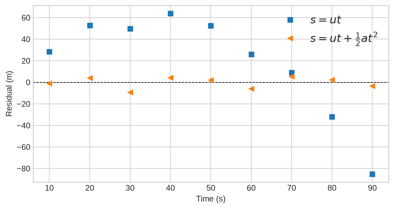

Figure 2: Residual plot of model minus data for the two fits

The constant-speed residuals form a clear arch — negative at short and long times, positive in the middle — which is the signature of a missing quadratic term. The constant-acceleration residuals scatter with no pattern, which is what a correct model should look like.

\(\chi^2\): quantifying how well a model fits

What \(\chi^2\) measures

curve_fit finds the best parameters by minimising the quantity

\[\chi^2 = \sum_{i=1}^{N} \frac{(y_i - f(x_i))^2}{\sigma_i^2}\]

Each term compares the squared residual \((y_i - f(x_i))^2\) to the squared measurement uncertainty \(\sigma_i^2\). If a residual is about the same size as the expected error, that term contributes roughly 1 to the sum. If a residual is much larger than the error, the term contributes much more, pulling \(\chi^2\) up. A lower \(\chi^2\) means the model is closer, on average, to each data point.

Note that \(\chi^2\) only has physical meaning when you used absolute_sigma=True. Without it, the sigma values were treated as relative weights and the covariance was rescaled — the \(\chi^2\) you calculate will not reflect your actual measurement precision.

Reduced chi-squared \(\chi_r^2\)

The raw \(\chi^2\) value grows with the number of data points, making it hard to compare fits across datasets. Dividing by the degrees of freedom (dof) produces the reduced chi-squared, whose ideal value is 1.0 regardless of the dataset size:

\[\chi_r^2 = \frac{\chi^2}{\text{dof}}, \qquad \text{dof} = N - m\]

where \(N\) is the number of data points and \(m\) is the number of fitted parameters. Each free parameter “uses up” one degree of freedom because the optimiser adjusts it to reduce \(\chi^2\).

Interpreting \(\chi_r^2\):

\(\chi_r^2 \approx 1\) — the residuals are about the same size as the measurement errors. This is exactly what you would expect from a correct model with correctly estimated errors.
\(\chi_r^2 \gg 1\) — the residuals are much larger than the measurement errors. Either the model is wrong (missing physics), the error estimates are too small, or there are outliers or systematic effects.
\(\chi_r^2 \ll 1\) — the residuals are much smaller than the measurement errors. Either the error estimates are too large (the experiment is more precise than you thought), or the model has too many parameters and is over-fitting the data.

def chi2(y_measure, y_predict, errors):
    """Chi-squared: sum of squared normalised residuals."""
    return numpy.sum((y_measure - y_predict)**2 / errors**2)

def chi2reduced(y_measure, y_predict, errors, number_of_parameters):
    """Reduced chi-squared."""
    dof = y_measure.size - number_of_parameters
    return chi2(y_measure, y_predict, errors) / dof

chi2r_linear = chi2reduced(measured_distances,
                            distance(measured_times, popt[0]),
                            distance_errors, 1)

chi2r_accel  = chi2reduced(measured_distances,
                            distance_with_acceleration(measured_times, popt2[0], popt2[1]),
                            distance_errors, 2)

print("Constant velocity model  χ²_r = {:.3g}".format(chi2r_linear))
print("Constant acceleration model χ²_r = {:.3g}".format(chi2r_accel))

Constant velocity model  χ²_r = 110
Constant acceleration model χ²_r = 1.18

Constant velocity model  χ²_r = 110.
Constant acceleration model χ²_r = 1.18

The constant-velocity model returns \(\chi_r^2 \approx 110\) — the residuals are about \(\sqrt{110} \approx 10\) times larger than the measurement errors. The constant-acceleration model returns \(\chi_r^2 \approx 1.2\), consistent with a good fit.

Reporting \(\chi_r^2\) values

Report \(\chi_r^2\) to 2–3 significant figures at most. Values of 110 and 1.18 should be rounded to 110 and 1.2 respectively:

print("χ²_r (linear)      =", round(chi2r_linear, -1))   # 110.0
print("χ²_r (acceleration)=", round(chi2r_accel,   1))   # 1.2

χ²_r (linear)      = 110.0
χ²_r (acceleration)= 1.2

\(\chi_r^2\) and the connection back to `absolute_sigma`

The \(\chi_r^2\) calculation and absolute_sigma=True are two sides of the same coin. When you use absolute_sigma=True, the uncertainties from pcov are physically meaningful, and the \(\chi_r^2\) you calculate has a clear interpretation: it tells you whether your measurement errors are consistent with your model. If you omit absolute_sigma=True, the default behaviour forces \(\chi_r^2 = 1\) internally by rescaling pcov, so calculating \(\chi_r^2\) afterwards with your original sigma values will give a meaningless number.

Challenge

Watching the parameters change

Put a print statement inside distance_with_acceleration to trace the parameter values during the fit. What is curve_fit doing?

Solution

def distance_with_acceleration_print(time, speed, acceleration):
    print("speed=", speed, "acceleration=", acceleration)
    return speed * time + 0.5 * acceleration * time**2

popt2, pcov2 = curve_fit(distance_with_acceleration_print,
                         measured_times, measured_distances,
                         absolute_sigma=True, sigma=distance_errors)

speed= 1.0 acceleration= 1.0
speed= 1.0000000149011612 acceleration= 1.0
speed= 1.0 acceleration= 1.0000000149011612
speed= 10.257717023172907 acceleration= 0.09589438502673808
speed= 10.257717176024801 acceleration= 0.09589438502673808
speed= 10.257717023172907 acceleration= 0.09589438645567577
speed= 10.257717029406022 acceleration= 0.09589438485479539

speed= 1.0 acceleration= 1.0
...
speed= 1.0000000149011612 acceleration= 1.0
speed= 1.0 acceleration= 1.0000000149011612
speed= 10.257717023193093 acceleration= 0.0958943850247661
...

curve_fit starts at the default guess (1, 1), then nudges each parameter slightly in turn to estimate the gradient of \(\chi^2\), then takes a step toward the minimum. The first three lines are the initial gradient estimate; the sudden jump to ≈ (10.3, 0.096) is the first large step; the remaining lines are fine adjustments converging on the minimum.

Non-linear models and the `p0` keyword

curve_fit works with any differentiable model — including non-linear ones such as \(y = a \, t^{\,b-1} + c\). The same chi2reduced and residual-plot checks apply.

For non-linear models the minimiser can get stuck in a local minimum if it starts too far from the true answer. The p0 keyword provides an initial guess:

No p0 defaults to all parameters equal to 1.0.
A rough physical estimate — order-of-magnitude, correct sign — is usually enough.
Being too precise is not necessary; the optimiser does the fine-tuning.
Being badly wrong (wrong sign, wrong order of magnitude) can cause the fit to diverge or converge to the wrong solution.

iteration = 0

def nonlinear_function(t, a, b, c, verbose=True):
    global iteration
    if verbose:
        print(iteration, "a=", a, "b=", b, "c=", c)
    iteration = iteration + 1
    return a * t**(b - 1) + c

t = numpy.arange(10)
y = numpy.array([-0.173, 2.12, 9.42, 19.69, 37.16, 59.40, 96.59, 119.448, 158.0, 201.9])
sigmaNL = numpy.ones(10) * 0.5

With a good guess the fit converges in ~14 iterations; with a bad guess the optimiser may diverge or converge to a wrong minimum entirely:

# Good guess: I think it's roughly 2.5*t^2 with no offset
iteration = 0
poptNL2, pcovNL2 = curve_fit(nonlinear_function, t, y,
                              absolute_sigma=True, sigma=sigmaNL, p0=(2.5, 3, 0))

# Bad guess: wrong sign on b
iteration = 0
poptNL3, pcovNL3 = curve_fit(nonlinear_function, t, y,
                              absolute_sigma=True, sigma=sigmaNL, p0=(3, -2, 0.1))

0 a= 2.5 b= 3.0 c= 0.0
1 a= 2.500000037252903 b= 3.0 c= 0.0
2 a= 2.5 b= 3.0000000447034836 c= 0.0
3 a= 2.5 b= 3.0 c= 1.4901161193847656e-08
4 a= 2.507540116653929 b= 2.9990074809599356 c= -0.9739171633288645
5 a= 2.507540154019188 b= 2.9990074809599356 c= -0.9739171633288645
6 a= 2.507540116653929 b= 2.9990075256486297 c= -0.9739171633288645
7 a= 2.507540116653929 b= 2.9990074809599356 c= -0.9739171488163678
8 a= 2.5074184209646457 b= 2.999031517139238 c= -0.973464273121737
9 a= 2.507418458328092 b= 2.999031517139238 c= -0.973464273121737
10 a= 2.5074184209646457 b= 2.99903156182829 c= -0.973464273121737
11 a= 2.5074184209646457 b= 2.999031517139238 c= -0.973464258615989
12 a= 2.5074214481566983 b= 2.999030967513556 c= -0.9734751858852739
0 a= 3.0 b= -2.0 c= 0.1
1 a= 3.0000000447034836 b= -2.0 c= 0.1
2 a= 3.0 b= -1.9999999701976776 c= 0.1
3 a= 3.0 b= -2.0 c= 0.10000000149011612

/tmp/ipykernel_2948/3523950367.py:8: RuntimeWarning: divide by zero encountered in power
  return a * t**(b - 1) + c
/tmp/ipykernel_2948/2588263260.py:8: OptimizeWarning: Covariance of the parameters could not be estimated
  poptNL3, pcovNL3 = curve_fit(nonlinear_function, t, y,

Always verify the result visually and with \(\chi_r^2\):

plt.figure(figsize=(8, 5))
plt.errorbar(t, y, yerr=sigmaNL, marker='o', ls='none', label="Data")

def plot_and_print(popt, ls, label):
    plt.plot(t, nonlinear_function(t, popt[0], popt[1], popt[2],
             verbose=False), label=label, ls=ls, lw=3)

plot_and_print(poptNL2, "--", "Good guess")
plot_and_print(poptNL3, ":",  "Bad guess")
plt.legend()
plt.xlabel("Time")
plt.ylabel("Value")
plt.show()

/tmp/ipykernel_2948/3523950367.py:8: RuntimeWarning: divide by zero encountered in power
  return a * t**(b - 1) + c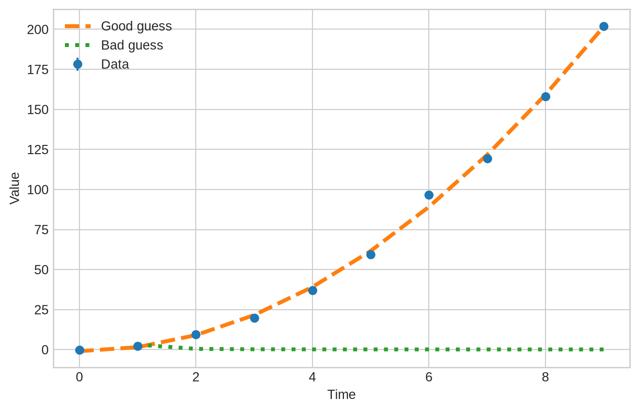

Figure 3: Two non-linear model fits overlaid on the data: a good initial guess that converges correctly and a bad initial guess that does not

plt.figure(figsize=(8, 4))
plt.axhline(0, color='k', lw=0.8, ls='--')

def plot_residual(data, popt, marker, label):
    plt.plot(t, nonlinear_function(t, popt[0], popt[1], popt[2],
             verbose=False) - data,
             label=label, marker=marker, ls='', lw=3)

plot_residual(y, poptNL2, "s", "Good guess")
plot_residual(y, poptNL3, "<", "Bad guess")
plt.legend()
plt.xlabel("Time (s)")
plt.ylabel("Residual")
plt.show()

/tmp/ipykernel_2948/3523950367.py:8: RuntimeWarning: divide by zero encountered in power
  return a * t**(b - 1) + c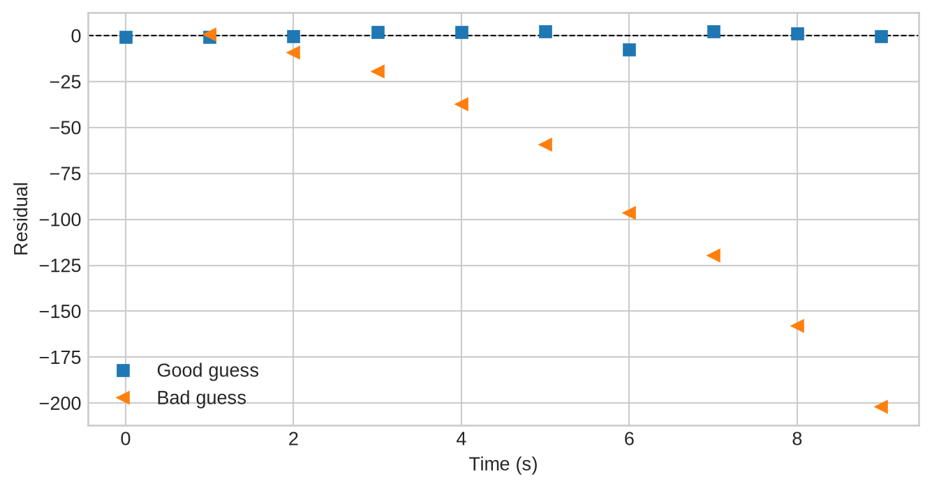

Figure 4: Residuals of the two non-linear fits

Key Points

curve_fit(model, x, y, sigma=errors, absolute_sigma=True) returns popt (best-fit parameters) and pcov (covariance matrix); use numpy.sqrt(numpy.diag(pcov)) for uncertainties.
Always use absolute_sigma=True when your sigma values represent real measurement errors in physical units.
Without absolute_sigma=True, curve_fit rescales uncertainties so that \(\chi_r^2 = 1\), which hides whether your model is actually a good fit.
Reduced chi-squared \(\chi_r^2 \approx 1\) indicates a good fit; \(\gg 1\) means the model or errors are wrong; \(\ll 1\) means errors are overestimated or the model is over-fit.
Residual plots reveal systematic trends invisible on the data plot; good residuals scatter randomly around zero with a spread matching the measurement errors.
For non-linear models, supply an initial guess with p0; always verify with a plot and \(\chi_r^2\).

Data analysis with Python

scipy.optimize.curve_fit fits a model function to data

popt and pcov: what curve_fit returns

sigma and absolute_sigma: getting uncertainties right

Predicting with the model

curve_fit works with multiple parameters

Always plot your data and model fits

Residual plots diagnose model quality

\(\chi^2\): quantifying how well a model fits

What \(\chi^2\) measures

Reduced chi-squared \(\chi_r^2\)

\(\chi_r^2\) and the connection back to absolute_sigma

Watching the parameters change

Non-linear models and the p0 keyword

`scipy.optimize.curve_fit` fits a model function to data

`popt` and `pcov`: what `curve_fit` returns

`sigma` and `absolute_sigma`: getting uncertainties right

`curve_fit` works with multiple parameters

\(\chi_r^2\) and the connection back to `absolute_sigma`

Non-linear models and the `p0` keyword