Root Finding by Iteration: Newton-Raphson

Questions

How does Newton-Raphson find the zero of a function by iteration?
How do I implement the iteration and detect when it has converged?
When does the method fail, and what do I do about it?

Objectives

Implement a Newton-Raphson loop in Python.
Apply it to find the zero of a transcendental equation from physics.
Visualise the iterative steps converging to the root.
Recognise convergence failure and use scipy.optimize as a robust alternative.

Why iterate?

Many physical equations have no closed-form solution. Setting the derivative of Planck’s spectral radiance to zero to find the peak wavelength leads to the transcendental equation:

\[5\left(1 - e^{-x}\right) = x \qquad x = \frac{hc}{\lambda_{\max} k T}\]

No algebraic manipulation will isolate x, but it can be solved by guessing a value of \(x\) (the left hand side), calculating a new value (the right hand side), and repeating.

Newton-Raphson is the standard choice when the function is smooth: starting from a guess \(x_0\), each step moves toward the root using the function value and its derivative:

\[x_{n+1} = x_n - \frac{f(x_n)}{f'(x_n)}\]

The method converges quadratically — the number of correct decimal places roughly doubles with each iteration.

Example problem: peak wavelength of the Sun

The Sun’s photosphere has an effective temperature of about 5778 K. At what wavelength does it emit most strongly? Wien’s displacement law gives \(\lambda_{\max} = b / T\), but the constant \(b\) must itself be found by solving the transcendental equation above.

Worked solution

Rewrite the equation as \(f(x) = 0\) and compute its derivative:

\[f(x) = 5\left(1 - e^{-x}\right) - x \qquad f'(x) = 5e^{-x} - 1\]

import numpy as np
import matplotlib.pyplot as plt

def f(x):
    return 5 * (1 - np.exp(-x)) - x

def f_prime(x):
    return 5 * np.exp(-x) - 1

Plot f(x) to confirm there is one physical root (the trivial root x = 0 is unphysical) and choose a starting guess:

x_vals = np.linspace(0.1, 8, 400)
plt.plot(x_vals, f(x_vals))
plt.axhline(0, color='k', linewidth=0.8, linestyle='--')
plt.xlabel("x")
plt.ylabel("f(x)")
plt.show()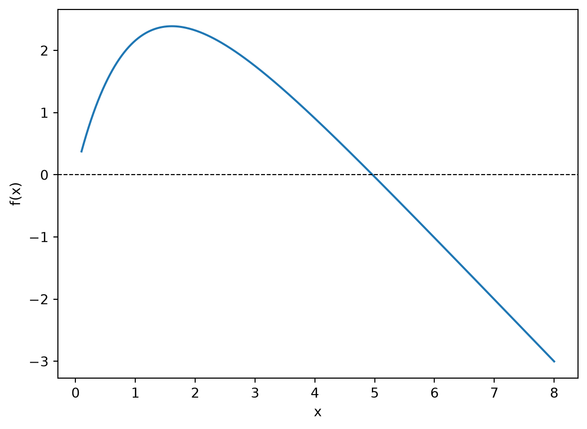

Figure 1: f(x) = 5(1 − e^{−x}) − x has a trivial root at x = 0 and the physical root near x ≈ 4.97

Run the Newton-Raphson iteration, recording each estimate so we can plot convergence:

x = 5.0          # starting guess, away from the trivial root at 0
tolerance = 1e-12
max_iter = 20
history = [x]

for i in range(max_iter):
    step = f(x) / f_prime(x)
    x = x - step
    history.append(x)
    if abs(step) < tolerance:
        print(f"Converged in {i+1} iterations")
        break

x_root = x
print(f"x root  = {x_root:.10f}")

Converged in 4 iterations
x root  = 4.9651142317

Convert the dimensionless root back to Wien’s displacement constant \(b = hc / (x k)\) and the peak wavelength of the Sun:

h = 6.626e-34   # J·s
c = 3.0e8       # m/s
k_B = 1.381e-23 # J/K
T_sun = 5778    # K

wien_b = h * c / (x_root * k_B)
lambda_max = wien_b / T_sun

print(f"Wien constant b  = {wien_b*1e6:.4f} μm·K  (accepted: 2897.8 μm·K)")
print(f"Peak wavelength  = {lambda_max*1e9:.1f} nm  (visible green-yellow)")

Wien constant b  = 2899.0103 μm·K  (accepted: 2897.8 μm·K)
Peak wavelength  = 501.7 nm  (visible green-yellow)

x_plot = np.linspace(3, 7, 300)
plt.plot(x_plot, f(x_plot), label="f(x)")
plt.axhline(0, color='k', linewidth=0.8, linestyle='--')

for n, xn in enumerate(history[:-1]):
    plt.plot(xn, f(xn), 'o', color=f'C{n+1}', markersize=6, label=f"$x_{n}$={xn:.3f}")

plt.axvline(x_root, color='r', linewidth=1, linestyle=':', label=f"root x = {x_root:.4f}")
plt.xlabel("x")
plt.ylabel("f(x)")
plt.legend(fontsize=8)
plt.show()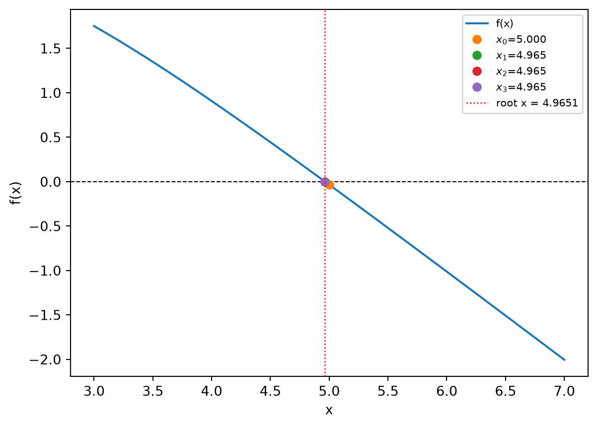

Figure 2: Each Newton-Raphson iterate plotted on f(x); the steps reach the root in just a few iterations

When Newton-Raphson fails

The method has two common failure modes:

Starting near the trivial root at x = 0: a guess below ~1 converges to 0 rather than to the physical root.
Derivative near zero: f′(x) = 5e^{−x} − 1 = 0 at x = ln 5 ≈ 1.61, directly between the two roots. Starting there causes a very large step.

For a guaranteed result, scipy.optimize.brentq only needs a bracket where f changes sign — no derivative required:

from scipy.optimize import brentq

# f(3) > 0 and f(6) < 0, confirmed by the plot above
x_brentq = brentq(f, 3.0, 6.0)
print(f"brentq:          x = {x_brentq:.10f}")
print(f"Newton-Raphson:  x = {x_root:.10f}")
print(f"Difference: {abs(x_brentq - x_root):.2e}")

brentq:          x = 4.9651142317
Newton-Raphson:  x = 4.9651142317
Difference: 0.00e+00

Both methods agree to full floating-point precision. brentq is easier to use if you can’t calculate a gradient for your function, and it’s safer if there are multiple roots or the starting location is not obvious. Newton-Raphson is useful when you want to inspect each iteration or when an analytic derivative is available and fast convergence matters.

Key Points

Rewrite the physical condition as \(f(x) = 0\) and compute \(f'(x)\) analytically.
Always plot \(f(x)\) first to count the roots and choose a starting guess away from trivial or spurious roots.
Newton-Raphson iterates \(x \leftarrow x - f(x)/f'(x)\) and converges quadratically — typically 5–10 iterations to machine precision.
scipy.optimize.brentq(f, a, b) is a robust fallback when a sign-changing bracket \([a, b]\) is available.