Solving Systems of Equations with scipy.fsolve

NoteQuestions
  • How do I find the value where two physical models agree?
  • How do I solve a system of two equations with two unknowns numerically?
NoteObjectives
  • Use scipy.optimize.fsolve to find the root of a single equation.
  • Extend fsolve to a system of two equations and two unknowns.
  • Recognise when a problem reduces to root-finding.

Why fsolve?

Many physics problems reduce to the question: at what value of x does f(x) = 0? Finding where two models agree — f(x) = g(x) — is equivalent to finding the root of h(x) = f(x) − g(x) = 0. scipy.optimize.fsolve solves this numerically for any differentiable function.

For a system of two equations in two unknowns, fsolve generalises: pass a function that returns a list of two residuals and an initial guess vector, and it returns the vector that makes both residuals zero.

Example problem: collision kinematics

Two pucks move along a frictionless track. Their positions are:

\[x_A(t) = 0.5 + 2.0\, t \qquad x_B(t) = 4.0 - 1.5\, t\]

At what time do they collide, and where?

Worked solution: single equation

import numpy as np
from scipy.optimize import fsolve
import matplotlib.pyplot as plt

def x_A(t): return 0.5 + 2.0 * t
def x_B(t): return 4.0 - 1.5 * t

# Collision means x_A(t) - x_B(t) = 0
def residual(t):
    return x_A(t) - x_B(t)

t_guess = 1.0
t_collision, = fsolve(residual, t_guess)
x_collision = x_A(t_collision)

print(f"Collision time:     {t_collision:.4f} s")
print(f"Collision position: {x_collision:.4f} m")
Collision time:     1.0000 s
Collision position: 2.5000 m
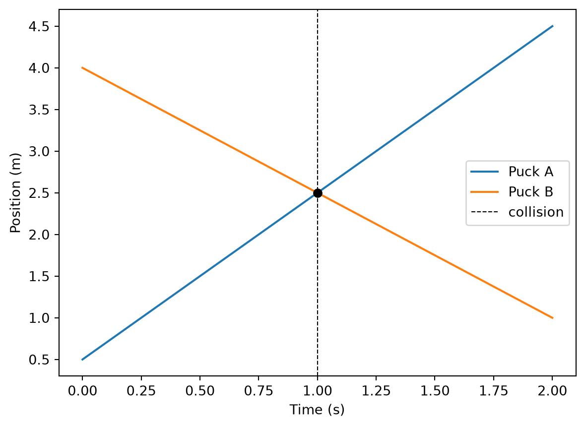
t = np.linspace(0, 2.0, 200)

plt.plot(t, x_A(t), label="Puck A")
plt.plot(t, x_B(t), label="Puck B")
plt.axvline(t_collision, color='k', linestyle='--', linewidth=0.8, label="collision")
plt.scatter([t_collision], [x_collision], zorder=5, color='k')
plt.xlabel("Time (s)")
plt.ylabel("Position (m)")
plt.legend()
plt.show()
Figure 1: Position versus time for pucks A and B; the intersection is the collision point found by fsolve

Extending to two unknowns: circuit currents

In a two-loop circuit with resistors R₁ = 2 Ω, R₂ = 3 Ω, R₃ = 1 Ω and voltage sources V₁ = 5 V, V₂ = 3 V, Kirchhoff’s voltage law gives:

\[ (R_1 + R_3)\,I_1 - R_3\,I_2 = V_1 \] \[ -R_3\,I_1 + (R_2 + R_3)\,I_2 = V_2 \]

Pass a function that returns the vector of residuals and an initial guess vector:

R1, R2, R3 = 2.0, 3.0, 1.0
V1, V2 = 5.0, 3.0

def circuit_residuals(currents):
    I1, I2 = currents
    eq1 = (R1 + R3) * I1 - R3 * I2 - V1
    eq2 = -R3 * I1 + (R2 + R3) * I2 - V2
    return [eq1, eq2]

I1, I2 = fsolve(circuit_residuals, [1.0, 1.0])
print(f"I1 = {I1:.4f} A")
print(f"I2 = {I2:.4f} A")
I1 = 2.0909 A
I2 = 1.2727 A

fsolve returns the vector [I₁, I₂] at which both residuals are zero — i.e., the solution to the system. For linear systems numpy.linalg.solve is more efficient, but fsolve works the same way when the equations become nonlinear.

TipKey Points
  • Rewrite f(x) = g(x) as h(x) = f(x) − g(x) = 0 and pass h to fsolve.
  • For two unknowns, return a two-element list from the residual function and pass a two-element initial guess.
  • Always plot the functions to check that your solution is at the right root and that the initial guess is reasonable.